Some time ago I wrote a post about Optimizing Java memory in Docker containers. I received a very interesting message regarding the impact Garbage Collector (GC) pauses can have on the behaviour of an application.

This message motivated me to write this post, where I will explain how GC can affect the performance of an application and how we can improve it by choosing the correct type of GC.

How Garbage Collector works?

GC plays a fundamental role within the JVM, since it is responsible for freeing up Heap Memory occupied by objects no longer in use in the application.

It normally works when the application reaches Heap Memory consumption levels close to the maximum available, at which point a GC cycle begins.

GC works following the Mark and Sweep algorithm. In the first instance, in the “Mark” phase, the object references in the Heap Memory are analyzed, marking reachable objects that is, accessible by the application. In the “Sweep” phase, GC reclaims Heap Memory space occupied by garbage (unreachable) objects, freeing up that space for new objects.

This allows developers to completely forget about memory management, which in turn causes them to lose control over memory, which could negatively affect application performance.

While GC is an implicit mechanism, Java offers different types of GC. Choosing the optimal one for each scenario improves application performance.

Serial Collector

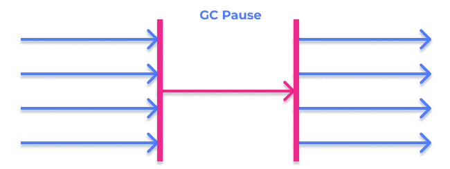
It is the simplest GC. It suspends all the threads of the application, to then execute the Mark and Sweep algorithm in a single thread. These GC-generated pauses in the application are known as “stop the world.”

Parallel Collector

This GC is similar to the previous one, with the difference that GC executes the Mark and Sweep algorithm on multiple threads. While there is still a pause in the application, its time is greatly reduced compared to the Serial Collector.

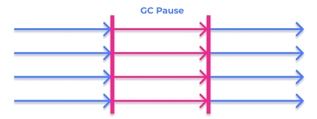
This type of GC is also known as a “Throughput Collector” as it is designed so that the application can provide high throughput.

Concurrent Collector

Concurrent Collector runs mostly at the same time as the application is running. This GC does not prevent pauses in the application and requires two short pauses compared to those generated by previous GCs.

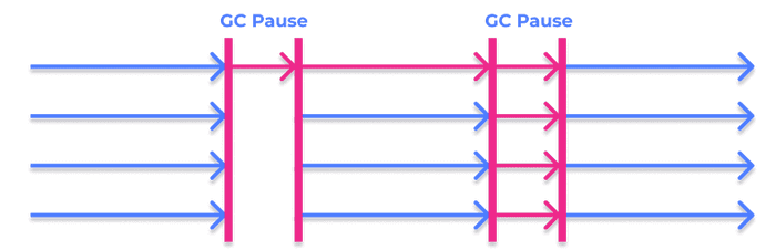
In the first pause, the “Mark” phase runs on the GC roots, which are the objects always accessible by the JVM from which references to other objects are generated in tree form.

The “Mark” phase continues concurrently with the application running, starting from the GC roots and marking the connected objects. Since objects are marked at the same time as application threads are running, new changes that may have been made to already marked objects are also recorded.

The second and final pause executes final markup on new objects that may have been created.

The starting Java application

In my previous post we saw how limiting the Heap Memory of a Java application can significantly reduce the total memory required. By monitoring the application after optimization, we verified that throughput remained the same as before optimization, even with a greater presence of GC due to the need to keep the Heap Memory consumption below the established limit.

While in the above scenario I didn’t find the need to do any GC-related optimization, what happens if we scale the same application and increase its load?

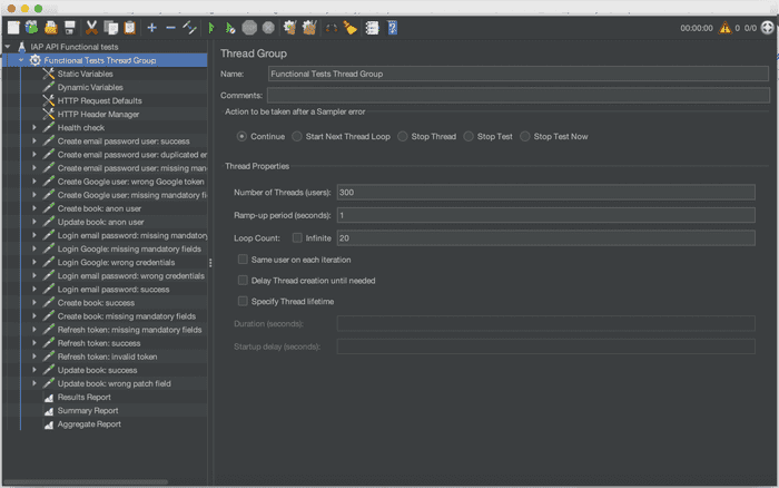
For this post I have scaled the application memory to support 300 active users simultaneously, which is three times more users than in the previous scenario.

Note that the GC type we are starting from is the Parallel Collector, which is the default GC in Java 8.

Monitoring tools

First, we are going to define the tools that we are going to use to monitor the application:

• Apache JMeter: to run a load test on the application and graphically view its performance.
• JConsole: to graphically view the Heap Memory and CPU consumption during the test.
• GCViewer: to graphically view logs generated by GC during the test.

Setting up JMeter

For the load test we start from the same JMeter project used in my previous post. The difference is that we modify the thread properties by configuring 300 simultaneous users instead of 100.

Now let’s configure JMeter to generate dashboards of our application performance during load testing. Fortunately, there is official documentation that explains how to configure this.

Setting up JConsole

To monitor the application with JConsole, the Java Management Extensions (JMX) must first be activated. In my previous post I explain step by step how to do it and how to connect JConsole to our application.

Setting up GC logs

GCViewer consumes GC logs file, therefore, before using GCViewer we have to configure the JVM to get GC logs.

The following JVM flags are needed for this:

• -XX:+PrintGCDetails: Activates the generation of detailed GC logs.
• -Xloggc:/tmp/gc/gc.log: Allows to specify the file path where to write GC logs.

With everything needed to run the load test, let’s do it!

Monitoring the application

Once the load test is finished, we will have the information available to understand how the application has behaved during the test.

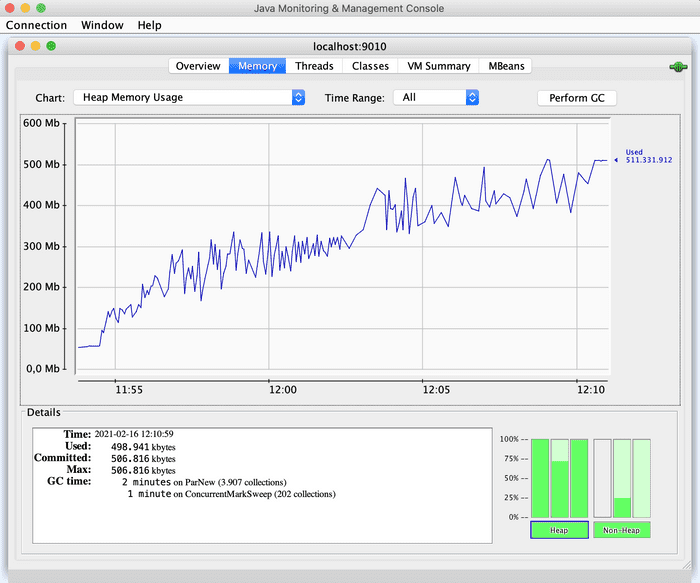
Let’s see in JConsole the Heap Memory consumption:

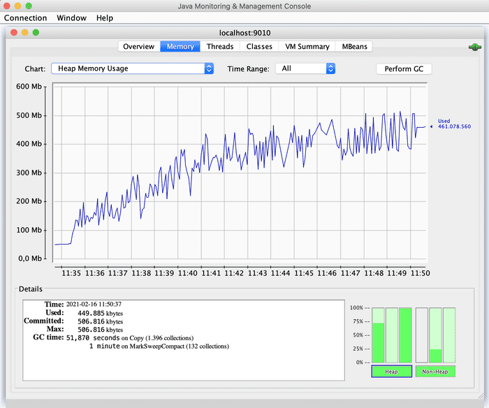
Heap memory consumption increases and stabilizes near 512Mb. This is because as the test progresses, Heap Memory takes care of new objects, ending up stabilizing near the established limit (512Mb). The peaks in the graph are due to the GC action.

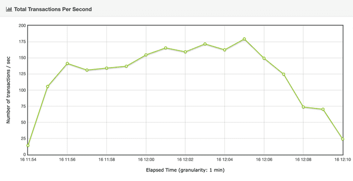
The next step is to analyze the application throughput. Let’s take a look at the JMeter generated dashboards:

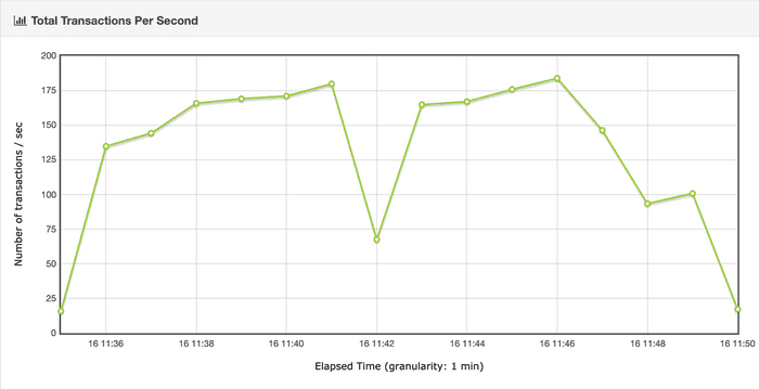
Throughput increases to about 175 transactions/second, dropping roughly in the seventh minute to about 70 transactions/second. This may be due to a pause caused by the GC, since it is Parallel. This hypothesis will be validated when we have analyzed the CG logs.

Drops like this can be unacceptable in applications where consistent high throughput is required.

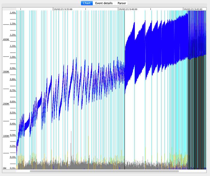
Next, we open the generated GC log file in GCViewer, to analyze GC behavior:

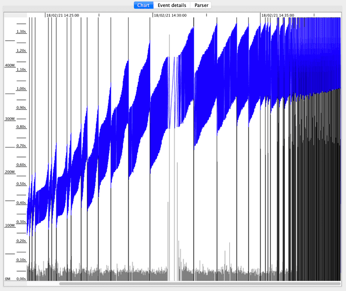
Vertical lines mark the start and end of a GC cycle. The frequency of GC cycles increases as the test progresses.

The blue areas correspond to the total Heap Memory used over time. The larger in use, the more GC cycles are required to free up space.

The dark gray lines at the bottom correspond to GC collection times. Collection times in the middle increase notably, is this related to the throughput drop?

GCViewer allows to expand the graph to monitor a more limited time interval. Let’s expand the graph to the seventh minute, to validate the hypothesis related to the throughput drop due to a possible GC pause.

Note that the dates and times shown in the schedule above do not correspond to those of the test, but are shown as if the test had started when the log file was opened in GCViewer. Fortunately, knowing the time interval, it is easy to place ourselves where we want.

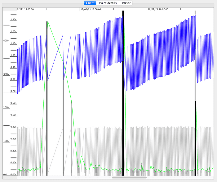
I enabled a GCViewer option that allows to view the GC times with green lines, since when enlarging the graph the information can be confusing.

We can see that we are positioned at the moment when GC collection time increases significantly, which also coincides with the throughput drop.

We confirm then that the hypothesis is true and that, therefore, throughput has been occasionally significantly affected by the CG type.

GCViewer also provides a table with aggregated GC performance data. The indicated throughput corresponds to the percentage of time that the application has not been busy with the GC, in our scenario 84.35%.

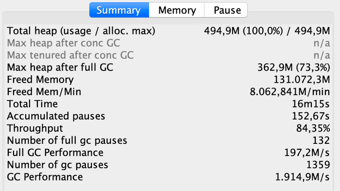
The information obtained is very useful for further GC optimizations. In this way, we can contrast the optimized GC performance with the initial scenario.

Now, what exactly are we going to do with the GC of the application?

As I mentioned earlier, in some scenarios we cannot afford throughput drops like the one above. However, the average throughput obtained, added to the percentage of time that the application has not been busy with GC, are more than acceptable results for other scenarios.

Suppose we need the application to be able to maintain a consistently good level of throughput, perhaps not as high as what Parallel Collector can offer, but without experiencing substantial drops. I’m sure many of you are already thinking that perhaps what we need is the Concurrent Collector.

Monitoring the application with Concurrent Collector

To benefit from this type of GC, we need to have multiple CPUs, otherwise this would not be the appropriate GC for our scenario.

On the other hand, due to the creation of new objects and changes in references between objects that can occur simultaneously with collections, this GC requires additional work that results in an increase in resource consumption.

With this in mind, let’s see how the application behaves with this GC!

First of all, it is necessary to configure the JVM to use the Concurrent Collector, so that it does not assign the default GC, which we remember is the Parallel Collector in our case. The JVM offers a specific flag for this: -XX:+UseConcMarkSweepGC.

Once the load test with Concurrent Collector has been executed, let’s analyze the graphs in this new scenario. We start with Heap Memory consumption:

Memory consumption increases in a similar way to the previous scenario until it approaches the maximum (512Mb), with the difference that the increases and decreases are shorter, due to the cleaning concurrent with the execution of the application.

Let’s see if thanks to the Concurrent Collector, we have avoided significant throughput drops:

During the test, throughput has remained at maximum values slightly lower than those obtained with the Parallel Collector, with the main advantage that we have not experienced any significant drop.

Let’s see in GCViewer how the Concurrent Collector has behaved:

The first thing that surely catches your eye in this graph are the vertical turquoise lines, which mark the collections made simultaneously by GC, something that does not exist in Parallel Collector.

The increases and decreases in Heap Memory consumption are more attenuated than in the Parallel Collector due to the concurrent collections.

Looking at the black lines that mark the beginning and end of the GC cycles, we see how, especially at the beginning of the test, they are longer in time.

Unlike what happened with Parallel Collector, there is no substantial increase in GC times.

To finish, let’s review the aggregated data table:

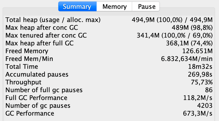
Throughput, which was 84.35% on the Parallel Collector, is now 75.73%, indicating that there has been a slightly higher GC occupation.

Which GC do we choose?

As I mentioned before, it depends on our scenario and application requirements.

With the Parallel Collector, the application can offer a very high throughput level at certain moments, although not sustainable over time, since it can experience significant drops due to GC pauses such as those in the test.

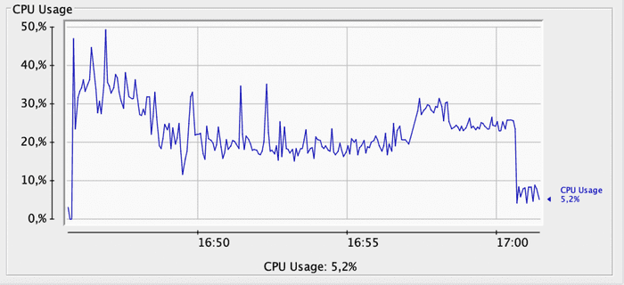
With the Concurrent Collector, slightly lower throughput is maintained on a sustained basis, although with an increase in CPU consumption. Below you can see a graph of the GC’s CPU consumption during the test:

And here, same graph using Parallel Collector:

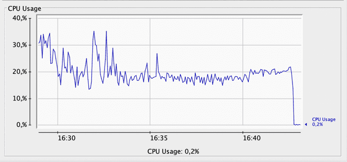
When comparing the two graphs, with the Concurrent Collector we see several CPU consumption peaks above 30%, some even exceeding 40%. With Parallel Collector, CPU consumption rarely exceeds 30%.

Taking the analysis into account, it is a matter of deciding which is the best option given our scenario and needs.

If we don’t need a particularly high level of throughput and we need to maintain it over time, the Concurrent Collector is a good choice, as long as we can handle the additional increase in CPU usage.

If we are looking to maximize the level of throughput, even if there may be significant drops, or we can’t assume the additional CPU consumption of the Concurrent Collector, opting for the Parallel Collector is a great idea.

To end…

In this post we have analyzed the performance of a Java application using different types of GC.

We have started from an example application that uses Parallel Collector as GC and analyzed the impact of this type of GC on the application performance with a load test, finding a high throughput level but with a significant drop due to a GC pause.

We then switched the GC type to Concurrent Collector and ran the same test, finding a slightly lower but sustainable level of throughput over time.

Finally, we compared the results obtained and we have identified the strengths and weaknesses of each CG to choose the optimal one for our scenario.

Please note that the results obtained in this analysis are specific to this scenario. In other scenarios you can find completely different results using the same GCs, so I recommend that you analyze your applications to find the type of GC that best suits your scenario.

Do you know other ways to optimize GC? I will be delighted if you tell me. Do not hesitate to contact me, also if you have any doubts that I can help you with ;)